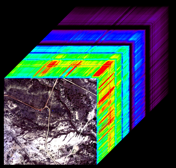
AVIRIS-NG Surface Spectral Reflectance#
Lessons learned working with the NSIDC dataset.
Dataset: SnowEx 2021; Senator Beck Basin and Grand Mesa
Tutorial Author: Brent Wilder
Learning Objectives
Understand how this data is structured
Understand where to find necessary terrain and illumination data
Learn about the
spectralpython package and apply it to this dataset
Computing environment#
We’ll be using the following open source Python libraries in this notebook:
from spectral import *
import numpy as np
import matplotlib.pyplot as plt
SnowEx21 Spectral Reflectance Dataset#
The data were collected using an airborne imaging spectrometer, AVIRIS-NG can be downloaded from here, https://nsidc.org/data/snex21_ssr/versions/1.
Reflectance is provided at 5 nm spectral resolution with a range of 380-2500 nm
For this dataset, the pixel resolution is 4 m
Data span from 19 March 2021 to 29 April 2021, and were collected in two snow-covered environments in Colorado: Senator Beck Basin and Grand Mesa
Each file will have a “.img” and “.hdr”. You need to have both of these in the same directory to open data.

Downloading necessary terrain and illumination data#
The NSIDC repository does not contain the terrain/illumination information.
However, you can obtain it for the matching flightline (by its timestamp) at the following URL, https://search.earthdata.nasa.gov/ ,
and searching for “AVIRIS-NG L1B Calibrated Radiance, Facility Instrument Collection, V1”
You only need to download the “obs_ort” files for the flight of interest. Please note these are different than “obs” files (ort means orthorectified).
In the Granule ID search, you can use wildcars “*” on either end of “obs_ort” to reduce your search.
You may also want to use this bounding box to reduce your search:
SW: 37.55725,-108.58887
NE: 39.78206,-106.16309
Using python package, spectral, to open data#
Important
Update the paths below to your local environment
# INSERT YOUR PATHS HERE
path_to_aviris = '/data/Albedo/AVIRIS/ang20210429t191025_rfl_v2z1'
path_to_aviris_hdr = '/data/Albedo/AVIRIS/ang20210429t191025_rfl_v2z1.hdr'
path_to_terrain = '/data/Albedo/AVIRIS/ang20210429t191025_rfl_v2z1_obs_ort'
path_to_terrain_hdr = '/data/Albedo/AVIRIS/ang20210429t191025_rfl_v2z1_obs_ort.hdr'
# Open a test image
aviris = envi.open(path_to_aviris_hdr)

# Save to an array in memory
rfl_array = aviris.open_memmap(writeable=True)

# print shape. You can see here we have 425 spectral bands for a grid of 1848x699 pixels
rfl_array.shape
(1848, 699, 425)
# You can create an array of the bands centers like this
bands = np.array(aviris.bands.centers)
bands
array([ 377.071821,  382.081821,  387.091821,  392.101821,  397.101821,
        402.111821,  407.121821,  412.131821,  417.141821,  422.151821,
        427.161821,  432.171821,  437.171821,  442.181821,  447.191821,
        452.201821,  457.211821,  462.221821,  467.231821,  472.231821,
        477.241821,  482.251821,  487.261821,  492.271821,  497.281821,
        502.291821,  507.301821,  512.301821,  517.311821,  522.321821,
        527.331821,  532.341821,  537.351821,  542.361821,  547.361821,
        552.371821,  557.381821,  562.391821,  567.401821,  572.411821,
        577.421821,  582.431821,  587.431821,  592.441821,  597.451821,
        602.461821,  607.471821,  612.481821,  617.491821,  622.491821,
        627.501821,  632.511821,  637.521821,  642.531821,  647.541821,
        652.551821,  657.561821,  662.561821,  667.571821,  672.581821,
        677.591821,  682.601821,  687.611821,  692.621821,  697.621821,
        702.631821,  707.641821,  712.651821,  717.661821,  722.671821,
        727.681821,  732.691821,  737.691821,  742.701821,  747.711821,
        752.721821,  757.731821,  762.741821,  767.751821,  772.751821,
        777.761821,  782.771821,  787.781821,  792.791821,  797.801821,
        802.811821,  807.821821,  812.821821,  817.831821,  822.841821,
        827.851821,  832.861821,  837.871821,  842.881821,  847.881821,
        852.891821,  857.901821,  862.911821,  867.921821,  872.931821,
        877.941821,  882.951821,  887.951821,  892.961821,  897.971821,
        902.981821,  907.991821,  913.001821,  918.011821,  923.021821,
        928.021821,  933.031821,  938.041821,  943.051821,  948.061821,
        953.071821,  958.081821,  963.081821,  968.091821,  973.101821,
        978.111821,  983.121821,  988.131821,  993.141821,  998.151821,
       1003.151821, 1008.161821, 1013.171821, 1018.181821, 1023.191821,
       1028.201821, 1033.211821, 1038.211821, 1043.221821, 1048.231821,
       1053.241821, 1058.251821, 1063.261821, 1068.271821, 1073.281821,
       1078.281821, 1083.291821, 1088.301821, 1093.311821, 1098.321821,
       1103.331821, 1108.341821, 1113.341821, 1118.351821, 1123.361821,
       1128.371821, 1133.381821, 1138.391821, 1143.401821, 1148.411821,
       1153.411821, 1158.421821, 1163.431821, 1168.441821, 1173.451821,
       1178.461821, 1183.471821, 1188.471821, 1193.481821, 1198.491821,
       1203.501821, 1208.511821, 1213.521821, 1218.531821, 1223.541821,
       1228.541821, 1233.551821, 1238.561821, 1243.571821, 1248.581821,
       1253.591821, 1258.601821, 1263.601821, 1268.611821, 1273.621821,
       1278.631821, 1283.641821, 1288.651821, 1293.661821, 1298.671821,
       1303.671821, 1308.681821, 1313.691821, 1318.701821, 1323.711821,
       1328.721821, 1333.731821, 1338.731821, 1343.741821, 1348.751821,
       1353.761821, 1358.771821, 1363.781821, 1368.791821, 1373.801821,
       1378.801821, 1383.811821, 1388.821821, 1393.831821, 1398.841821,
       1403.851821, 1408.861821, 1413.861821, 1418.871821, 1423.881821,
       1428.891821, 1433.901821, 1438.911821, 1443.921821, 1448.931821,
       1453.931821, 1458.941821, 1463.951821, 1468.961821, 1473.971821,
       1478.981821, 1483.991821, 1488.991821, 1494.001821, 1499.011821,
       1504.021821, 1509.031821, 1514.041821, 1519.051821, 1524.061821,
       1529.061821, 1534.071821, 1539.081821, 1544.091821, 1549.101821,
       1554.111821, 1559.121821, 1564.121821, 1569.131821, 1574.141821,
       1579.151821, 1584.161821, 1589.171821, 1594.181821, 1599.191821,
       1604.191821, 1609.201821, 1614.211821, 1619.221821, 1624.231821,
       1629.241821, 1634.251821, 1639.251821, 1644.261821, 1649.271821,
       1654.281821, 1659.291821, 1664.301821, 1669.311821, 1674.321821,
       1679.321821, 1684.331821, 1689.341821, 1694.351821, 1699.361821,
       1704.371821, 1709.381821, 1714.381821, 1719.391821, 1724.401821,
       1729.411821, 1734.421821, 1739.431821, 1744.441821, 1749.451821,
       1754.451821, 1759.461821, 1764.471821, 1769.481821, 1774.491821,
       1779.501821, 1784.511821, 1789.511821, 1794.521821, 1799.531821,
       1804.541821, 1809.551821, 1814.561821, 1819.571821, 1824.581821,
       1829.581821, 1834.591821, 1839.601821, 1844.611821, 1849.621821,
       1854.631821, 1859.641821, 1864.651821, 1869.651821, 1874.661821,
       1879.671821, 1884.681821, 1889.691821, 1894.701821, 1899.711821,
       1904.711821, 1909.721821, 1914.731821, 1919.741821, 1924.751821,
       1929.761821, 1934.771821, 1939.781821, 1944.781821, 1949.791821,
       1954.801821, 1959.811821, 1964.821821, 1969.831821, 1974.841821,
       1979.841821, 1984.851821, 1989.861821, 1994.871821, 1999.881821,
       2004.891821, 2009.901821, 2014.911821, 2019.911821, 2024.921821,
       2029.931821, 2034.941821, 2039.951821, 2044.961821, 2049.971821,
       2054.971821, 2059.981821, 2064.991821, 2070.001821, 2075.011821,
       2080.021821, 2085.031821, 2090.041821, 2095.041821, 2100.051821,
       2105.061821, 2110.071821, 2115.081821, 2120.091821, 2125.101821,
       2130.101821, 2135.111821, 2140.121821, 2145.131821, 2150.141821,
       2155.151821, 2160.161821, 2165.171821, 2170.171821, 2175.181821,
       2180.191821, 2185.201821, 2190.211821, 2195.221821, 2200.231821,
       2205.231821, 2210.241821, 2215.251821, 2220.261821, 2225.271821,
       2230.281821, 2235.291821, 2240.301821, 2245.301821, 2250.311821,
       2255.321821, 2260.331821, 2265.341821, 2270.351821, 2275.361821,
       2280.361821, 2285.371821, 2290.381821, 2295.391821, 2300.401821,
       2305.411821, 2310.421821, 2315.431821, 2320.431821, 2325.441821,
       2330.451821, 2335.461821, 2340.471821, 2345.481821, 2350.491821,
       2355.491821, 2360.501821, 2365.511821, 2370.521821, 2375.531821,
       2380.541821, 2385.551821, 2390.561821, 2395.561821, 2400.571821,
       2405.581821, 2410.591821, 2415.601821, 2420.611821, 2425.621821,
       2430.621821, 2435.631821, 2440.641821, 2445.651821, 2450.661821,
       2455.671821, 2460.681821, 2465.691821, 2470.691821, 2475.701821,
       2480.711821, 2485.721821, 2490.731821, 2495.741821, 2500.751821])
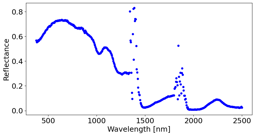
# A simple data visalization by selecting random indices
i = 900
j = 300
pixel = rfl_array[i,j,:]

fig, ax = plt.subplots(1, 1, figsize=(10,5))
plt.rcParams.update({'font.size': 18})
ax.scatter(bands, pixel, color='blue', s=20)
ax.set_xlabel('Wavelength [nm]')
ax.set_ylabel('Reflectance')
plt.show()

Lastly, a very important note!#
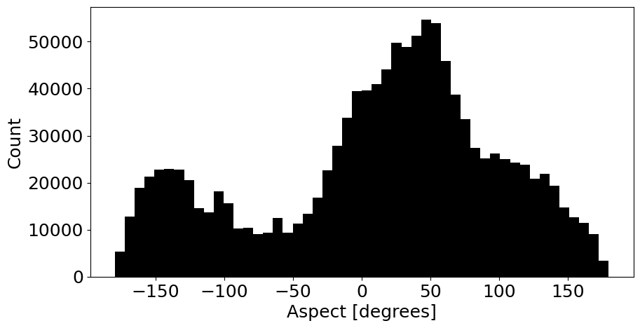
Please notice that convention for aspect follows \(-\pi\) to \(\pi\).
# Terrain bands:
# 0 - Path length (m)
# 1 - To sensor azimuth
# 2 - To sensor zenith
# 3 - To sun azimuth
# 4 - To sun zenith
# 5 - Solar phase
# 6 - Slope
# 7 - Aspect
# 8 - cosine(i) (local solar illumination angle)
# 9 - UTC Time
# 10 - Earth-sun distance (AU)

# open envi object
terrain = envi.open(path_to_terrain_hdr)

# Save to an array in memory
terrain_array = terrain.open_memmap(writeable=True)

# Grab just aspect and flatten (remove nan)
aspects = terrain_array[:,:,7].flatten()
aspects = aspects[aspects>-9999]


# Plot a histogram to show aspect range
fig, ax = plt.subplots(1, 1, figsize=(10,5))
plt.rcParams.update({'font.size': 18})
ax.hist(aspects, color='black', bins=50)
ax.set_xlabel('Aspect [degrees]')
ax.set_ylabel('Count')
plt.show()

References#
To further explore these topics:

