Data Exploration

Data Exploration#

(15 minutes)

Prerequisites: an EarthData Login

Learning Objectives

Experience a variety of SnowEx data across different spatial and temporal domains
Preview code snippets to help you extract and prep data
Get a first taste of the database!

PART I: Spatial Data#

Let’s take a look at data collected during the Intense Observation Periods (IOP) campaigns via EarthAcess data downloads.

I: 2017/2020 - Grand Mesa & Senator Beck, Colorado#

Objective - Visualize SWE from Grand Mesa field campaigns.
Data description - SnowEx 2017 & 2020 IOP derived SWE from snow pits.
Datasets -

SnowEx17 Community Snow Pit Measurements, Version 1 (Grand Mesa + Senator Beck, CO)
SnowEx20 Grand Mesa Intensive Observation Period Snow Pit Measurements, Version 1 (Grand Mesa, CO)

We will begin by importing python packages we will need to explore data.

# standard imports
import pandas as pd
import pyproj
import datetime

# plotting imports
import matplotlib
import matplotlib.pyplot as plt
# from matplotlib import gridspec # do I use?
import matplotlib.dates as mdates
# import matplotlib.patches as patches # do I use?
import seaborn as sns

# mapping imports
import folium
from pyproj import Transformer
import branca.colormap as cm
from folium import IFrame
from folium.plugins import MeasureControl

# Earthaccess imports
import earthaccess

Now we continue by accessing data with our EarthData accounts from NSIDC.

Download data from NASA’s NSIDC DAAC#

# connect to Earthaccess
auth = earthaccess.login()

From EarthData we can glean information about the files we are interested in. For example, we learn that the SnowEx 2017 snow pit data are a multi-file granule, which will require one extra step to download.

# pull SnowEx 2017 snow pit data - Summary_SWE file
results_gm17 =earthaccess.search_data(
    short_name='SNEX17_SNOWPITS',
    granule_name = 'SnowEx17_SnowPits_GM')

# some extra code to filter a multi-file granule (2017 IOP granules: 1). SnowEx17_SnowPits_GM, 2). SnowEx17_SnowPits_SBB
filtered_urls = []

for granule in results_gm17:
    links = granule.data_links()
    for link in links:
        if link == 'https://n5eil01u.ecs.nsidc.org/DP1/SNOWEX/SNEX17_SnowPits.001/2017.02.06/SnowEx17_SnowPits_GM_201702_v01.csv':
            filtered_urls.append(link) # Knowing the name of the file I wanted helped here

earthaccess.download(filtered_urls, 
                     local_path='./Downloads')

['Downloads/SnowEx17_SnowPits_GM_201702_v01.csv']

# pull SnowEx 2020 snow pit data - Summary_SWE file
results_gm20 =earthaccess.search_data(
    short_name='SNEX20_GM_SP',
    granule_name = 'SnowEx20_SnowPits_GMIOP_Summary_SWE_2020_v01.csv')

downloaded_file_gm20 = earthaccess.download(
    results_gm20,
    local_path='./Downloads',
)

Note

The downside to this method is you have to know the specific filename you are interested in. That can require more time to familiarize yourself with the dataset. A great resource is to read the User Guide provided for most SnowEx data sets and accessed from the NSIDC data landing page. The User Guides provide information about filenames.

Look over to the left in your files and see that we added a ./Downloads folder to store the EarthData download.

Next, let’s use Python’s pandas package to open the CSV file that contains Summary SWE data.

# open summary SWE files from our ./Downloads folder
s17 = pd.read_csv('./Downloads/SnowEx17_SnowPits_GM_201702_v01.csv')
s20 = pd.read_csv('./Downloads/SnowEx20_SnowPits_GMIOP_Summary_SWE_2020_v01.csv')

print(s17.info())
s17.describe()

<class 'pandas.core.frame.DataFrame'>
RangeIndex: 264 entries, 0 to 263
Data columns (total 13 columns):
 #   Column                   Non-Null Count  Dtype 
---  ------                   --------------  ----- 
 0   #Location                264 non-null    object
 1   Site                     264 non-null    object
 2   PitID                    264 non-null    object
 3   Date/Time (MST)          264 non-null    object
 4   UTM13 Easting [m]        264 non-null    int64 
 5   UTM13 Northing [m]       264 non-null    int64 
 6   Density A Mean [kg/m^3]  264 non-null    int64 
 7   Density B Mean [kg/m^3]  264 non-null    int64 
 8   Density Mean [kg/m^3]    264 non-null    int64 
 9   SWE A [mm]               264 non-null    int64 
 10  SWE B [mm]               264 non-null    int64 
 11  SWE [mm]                 264 non-null    int64 
 12  Snow Depth [cm]          264 non-null    int64 
dtypes: int64(9), object(4)
memory usage: 26.9+ KB
None

	UTM13 Easting [m]	UTM13 Northing [m]	Density A Mean [kg/m^3]	Density B Mean [kg/m^3]	Density Mean [kg/m^3]	SWE A [mm]	SWE B [mm]	SWE [mm]	Snow Depth [cm]
count	264.000000	2.640000e+02	264.000000	264.000000	264.000000	264.000000	264.000000	264.000000	264.000000
mean	239602.007576	4.306328e+06	322.227273	322.840909	322.515152	472.484848	473.253788	472.901515	145.856061
std	12054.013830	4.553288e+04	17.479849	17.394475	17.289081	123.046437	122.673637	122.774817	34.450412
min	221314.000000	4.196923e+06	254.000000	263.000000	258.000000	114.000000	118.000000	116.000000	45.000000
25%	232181.000000	4.322908e+06	313.000000	312.000000	312.000000	399.500000	399.000000	400.000000	126.000000
50%	236112.500000	4.324478e+06	321.000000	322.000000	321.000000	476.000000	477.000000	477.000000	148.500000
75%	249477.500000	4.326407e+06	332.000000	334.250000	334.000000	559.000000	563.250000	560.000000	169.000000
max	261866.000000	4.332499e+06	371.000000	371.000000	371.000000	952.000000	952.000000	952.000000	257.000000

# some dataframe clean up
s17 = s17[s17['#Location'] == 'GM-CO'] # keep the GM points only for now
s20 = s20[s20['Easting (m)'] < 750000] # removes point at GM lodge (n=1)

# Convert UTM to Lat/Lon
transformer = pyproj.Transformer.from_crs("EPSG:32613", "EPSG:4326") # UTM Zone 13N 
s17['latitude'], s17['longitude'] = zip(*s17.apply(lambda row: transformer.transform(row['UTM13 Easting [m]'], row['UTM13 Northing [m]']), axis=1))

transformer = pyproj.Transformer.from_crs("EPSG:32612", "EPSG:4326") # UTM Zone 12N
s20['latitude'], s20['longitude'] = zip(*s20.apply(lambda row: transformer.transform(row['Easting (m)'], row['Northing (m)']), axis=1))

Now that we have added Latitude and Longitude columns, let’s look at the spatial extent of the data.

fig, ax = plt.subplots(figsize=(8,4))
s17.plot.scatter('latitude', 'longitude', color='blueviolet', ax=ax, label='GrandMesa 2017')
s20.plot.scatter('latitude', 'longitude', color='orange', ax=ax, label='GrandMesa 2020')
plt.legend(loc='lower right')
plt.show()

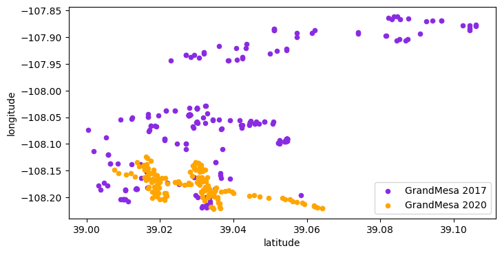
../../_images/da209cb408805831142f761e37e435cac9e61b1034b8db15780797593d217522.png

We see that during the 2017 IOP the sampling area covered a greater extent.

Let’s add some context to these data points#

By using an interactive map (Folium) we can move around the Mesa. Here we plot Latitude and Longitude on the y- and x-axes, respectively and add plot SWE as the 3rd dimension with the additional of a colorbar.

# Create a map using lat/lon mean
m = folium.Map(width=500, height=400,location=[s17['latitude'].mean(), s17['longitude'].mean()], zoom_start=10)
m

Make this Notebook Trusted to load map: File -> Trust Notebook

I used the dataframe’s lat/lon mean to center my map. I choose the 2017 dataframe because of the greater spatial extent we discovered above.

Let’s now modify the map imagery

# Add aerial imagery (ESRI World Imagery)
folium.TileLayer(
    tiles='https://server.arcgisonline.com/ArcGIS/rest/services/World_Imagery/MapServer/tile/{z}/{y}/{x}',
    attr='Esri',
    name='Esri Satellite',
    overlay=False,
    control=True,
    opacity=0.9
).add_to(m)

m

Make this Notebook Trusted to load map: File -> Trust Notebook

Oh goody, I can see the Mesa! Did you know this is the largest flat-topped mountain in the world? See for yourself right here.

Moving on, let’s add the SWE values to the map!

Map + Imagery + Data#

# Create a Folium map 
m = folium.Map(width=1000, height=600, location=[s17['latitude'].mean(), s17['longitude'].mean()], zoom_start=10)

# Add aerial imagery (ESRI World Imagery)
folium.TileLayer(
    tiles='https://server.arcgisonline.com/ArcGIS/rest/services/World_Imagery/MapServer/tile/{z}/{y}/{x}',
    attr='Esri',
    name='Esri Satellite',
    overlay=False,
    control=True,
    opacity=0.9
).add_to(m)

# Create a colormap 
colormap1 = cm.linear.Purples_09.to_step(12).scale(50,800)
colormap2 = cm.linear.YlOrBr_04.to_step(12).scale(50,800)

# Plot the scatter plot for s17
for index, row in s17.iterrows():
    folium.CircleMarker(location=[row['latitude'], row['longitude']], radius=3, fill=True, fill_opacity=1, color=colormap1(row['SWE [mm]'])).add_to(m)

# Plot the scatter plot for s20
for index, row in s20.iterrows():
    folium.CircleMarker(location=[row['latitude'], row['longitude']], radius=3, fill=True, fill_opacity=1, color=colormap2(row['SWE Mean (mm)'])).add_to(m)

# Add colorbar legend to the map
colormap1.add_to(m)
colormap1.caption = '2017 SWE (mm)'
colormap1.stroke_color = '#ffffff'  # White color for the text buffer

colormap2.add_to(m)
colormap2.caption = '2020 SWE (mm)'
colormap2.stroke_color = '#ffffff'  # White color for the text buffer

# Define custom CSS for the colorbar legend
custom_css = """
<style>
    .legend {
        font-size: 16px !important;
        height: 80px !important;  /* Adjust the height of the colorbar */
    }
    .legend .caption {
        font-size: 18px !important;
        font-weight: bold;
        text-shadow: 0 0 3px #ffffff;
    }
    .legend .min, .legend .max {
        font-size: 16px !important;
        text-shadow: 0 0 3px #ffffff;
    }
</style>
"""

m.add_child(MeasureControl(position='bottomleft', primary_length_unit='meters', secondary_length_unit='miles', primary_area_unit='sqmeters', secondary_area_unit='acres'))

# Add the custom CSS to the map
m.get_root().html.add_child(folium.Element(custom_css))

# Save the map as an HTML file or display it in Jupyter notebook
# m.save(path_out.joinpath('GMIOP_20_swe_map.html'))

# Display the map
m

Make this Notebook Trusted to load map: File -> Trust Notebook

Note

The Grand Mesa plateau splits the 12 & 13 UTM zone. That means the western portion of the Mesa is Zone 12 while the eastern portion is Zone 13. Due to the sampling design, the SnowEx 2017 data were collected as Zone 13 (majority of points were east of the divide) and SnowEx 2020 data were collected as Zone 12 (majority of points focused on the western portion of the plateau).

What variability is there during the different sampling years?#

# open again to reset (recall, we filtered out Senator Beck data before, let's keep that this time!)
s17 = pd.read_csv('./Downloads/SnowEx17_SnowPits_GM_201702_v01.csv')
s20 = pd.read_csv('./Downloads/SnowEx20_SnowPits_GMIOP_Summary_SWE_2020_v01.csv')

# subdataframes for GM and SB for 2017
s17_gm = s17[s17['#Location'] == 'GM-CO'] 
s17_sb = s17[s17['#Location'] == 'SBB-CO'] 

fig, axs = plt.subplots(1, 2, figsize=(12, 5))

# ~~~~ Plot 1: Scatter plot of density and SWE for S17 and S20

# Count the number of observations
n_s17_sb = s17_sb['SWE [mm]'].count()
n_s17_gm = s17_gm['SWE [mm]'].count()
n_s20 = s20['SWE Mean (mm)'].count()

# Plot data for 2017 SBB
sns.scatterplot(data=s17_sb, x='Density Mean [kg/m^3]', y='Snow Depth [cm]', s=60, label=f'2017 SBB-CO (n={n_s17_sb})', marker='^', ax=axs[0])

# Plot data for 2017 GM
sns.scatterplot(data=s17_gm, x='Density Mean [kg/m^3]', y='Snow Depth [cm]', s=60, label=f'2017 GM-CO (n={n_s17_gm})', marker='^', ax=axs[0])

# Plot data for 2020 GM
sns.scatterplot(data=s20, x='Density Mean (kg/m^3)', y='Snow Depth (cm)', s=40, label=f'2020 GM-CO (n={n_s20})', ax=axs[0])

# Adding labels and legends
axs[0].set_xlabel('Snow Density (kg/m$^3$)')
axs[0].set_ylabel('Snow Depth (cm)')
axs[0].legend()
axs[0].set_title('S17 and S20 Snow Pit Bulk Density and Depth')
axs[0].grid(True)


# ~~~~ Plot 2: PDF for S17 (Grand Mesa + Senator Beck) and S20 (Grand Mesa 2020)

# Plot the PDF for 2017 SBB
sns.kdeplot(s17_sb['SWE [mm]'], label='2017 SBB-CO', linewidth=5, ax=axs[1])

# Plot the PDF for 2017 GM
sns.kdeplot(s17_gm['SWE [mm]'], label='2017 GM-CO', linewidth=5, ax=axs[1])

# Plot the PDF for 2020 GM
sns.kdeplot(s20['SWE Mean (mm)'], label='2020 GM-CO', linewidth=5, ax=axs[1])

# Add title and labels
axs[1].set_title('S17 and S20 Snow Pit SWE')
axs[1].set_xlabel('SWE (mm)')
axs[1].set_ylabel('PDF')
axs[1].legend()

# Save figure if needed
# plt.savefig(path_fig.joinpath('S17_n_S20_GMIOP_pdf.jpg'), bbox_inches='tight', pad_inches=0.1)

# Show the plot
plt.tight_layout()
plt.show()

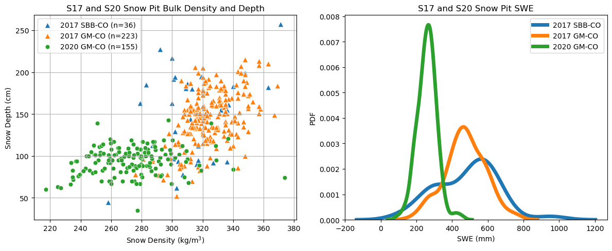
../../_images/bd71206e21228a53acd4ce1de3e96eb363564ce62eb13e5884e127ec3c172a8b.png

There is so much more we could dig into. Just ask HP, he’ll say you could spend a lifetime studying snow on Grand Mesa :)

Alas, let us continue our spatial exploration but move it up to Alaska.

II: 2023 Arctic Tundra and Boreal Forest, Alaska#

Objectives:

Compare snow depth, density and SWE data from the Adirondack snow sampler (n=84) and snow pits (n=170)
Explore data within the snowexsql database Data description - SnowEx 2023 March 2023 IOP Snow Water Equivalent and Snow Pit Measurements\

Datasets -

SnowEx23 Snow Water Equivalent, Version 1 (2-days of Adirondack snow sampler measurements North Slope (tundra) and Fairbanks (boreal forest))
SnowEx23 Snow Pit Measurements, Version 1 (in prep., available on the snowexsql database)

# Adirondack SWE download
results_swe = earthaccess.search_data(
    short_name='SNEX23_SWE')

downloaded_files_swe = earthaccess.download(
    results_swe,
    local_path='./Downloads',
)

# datasets from Alaska contain more header rows. skipping 42 rows for now and dropping the numbered row under the columns names
s23 = pd.read_csv('./Downloads/SNEX23_SWE_Mar23IOP_AK_20230313_20230316_v01.0.csv', header=42, na_values=-9999)
s23 = s23.iloc[1:] # selects the row below the header number cols(1, 2, 3, ... etc.)
s23 = s23.reset_index(drop=True)
s23['County'] = s23['County'].replace({'Fairbanks': 'FLCF \n(Boreal Forest)', 'North Slope': 'UKT \n(Arctic Tundra)'})

s23.head()

	State	County	Site ID	Latitude	Longitude	Elevation	Date	Depth1	Depth2	Depth3	Mass1	Mass2	Mass3	Density1	Density2	Density3	SWE1	SWE2	SWE3
0	Alaska	UKT \n(Arctic Tundra)	UKE1	68.611087	-149.493961	963	13-Mar-23	34	32.0	32.0	198	190.0	209.0	163	166.0	183.0	55	53.0	59.0
1	Alaska	UKT \n(Arctic Tundra)	UKE1.5	68.611280	-149.481889	942	13-Mar-23	72	76.0	74.0	645	663.0	584.0	251	244.0	303.0	181	186.0	164.0
2	Alaska	UKT \n(Arctic Tundra)	UKE2	68.611497	-149.470469	935	13-Mar-23	97	102.0	101.0	839	891.0	917.0	242	245.0	254.0	235	250.0	257.0
3	Alaska	UKT \n(Arctic Tundra)	UKE2.5	68.611411	-149.459072	951	13-Mar-23	32	20.0	12.0	188	91.0	85.0	165	127.0	198.0	53	25.0	24.0
4	Alaska	UKT \n(Arctic Tundra)	UKE3	68.611550	-149.447256	938	13-Mar-23	68	68.0	68.0	502	484.0	470.0	207	201.0	197.0	141	137.0	134.0

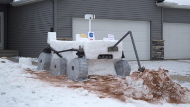
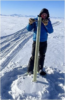
At each coordinate pair, the Adirondack snow sampler (i.e a large SWE tube, cross-sectional area A = 35.7 cm2) is used to collect 3 samples each of depth (cm) and mass (g). Bulk snow density and SWE are then computed afterwards using the equations from Stuefer et al., 2020. Here is the device being used on the North Slope in Alaska.

Okay, back to some data analysis.

# CREATE DEPTH, DENSITY, and SWE Boxplots with the SWE Adirondack snow sampler

# Combine the SWE, Depth, and Density columns for plotting (3 samples/location)
df_melted = pd.melt(s23, id_vars=['State', 'County'], value_vars=['SWE1', 'SWE2', 'SWE3', 'Depth1', 'Depth2', 'Depth3', 'Density1', 'Density2', 'Density3'],
                    var_name='Measurement', value_name='Value')

# Create sub-dataframes for SWE, Depth, and Density
swe_df = df_melted[df_melted['Measurement'].str.contains('SWE')]
depth_df = df_melted[df_melted['Measurement'].str.contains('Depth')]
density_df = df_melted[df_melted['Measurement'].str.contains('Density')]

# Initialize the figure and axes
fig, axs = plt.subplots(1, 3, figsize=(14, 6))

# Define the custom order and labels
custom_order = ['FLCF \n(Boreal Forest)', 'UKT \n(Arctic Tundra)']

# Plot the SWE boxplot
sns.boxplot(data=swe_df, x='County', y='Value', ax=axs[0], color='gray', order=custom_order)
axs[0].set_title('SWE')
axs[0].set_ylabel('SWE (mm)')

# Plot the Depth boxplot
sns.boxplot(data=depth_df, x='County', y='Value', ax=axs[1], color='gray', order=custom_order)
axs[1].set_title('Depth')
axs[1].set_ylabel('Depth (cm)')

# Plot the Density boxplot
sns.boxplot(data=density_df, x='County', y='Value', ax=axs[2], color='gray', order=custom_order)
axs[2].set_title('Density')
axs[2].set_ylabel('Density (kg/m$^3$)')

# Adjust the layout
plt.tight_layout()
plt.show()

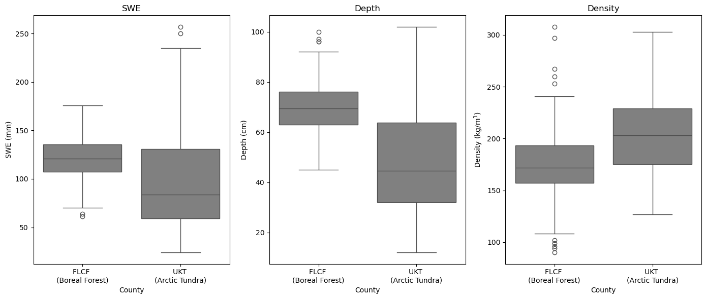
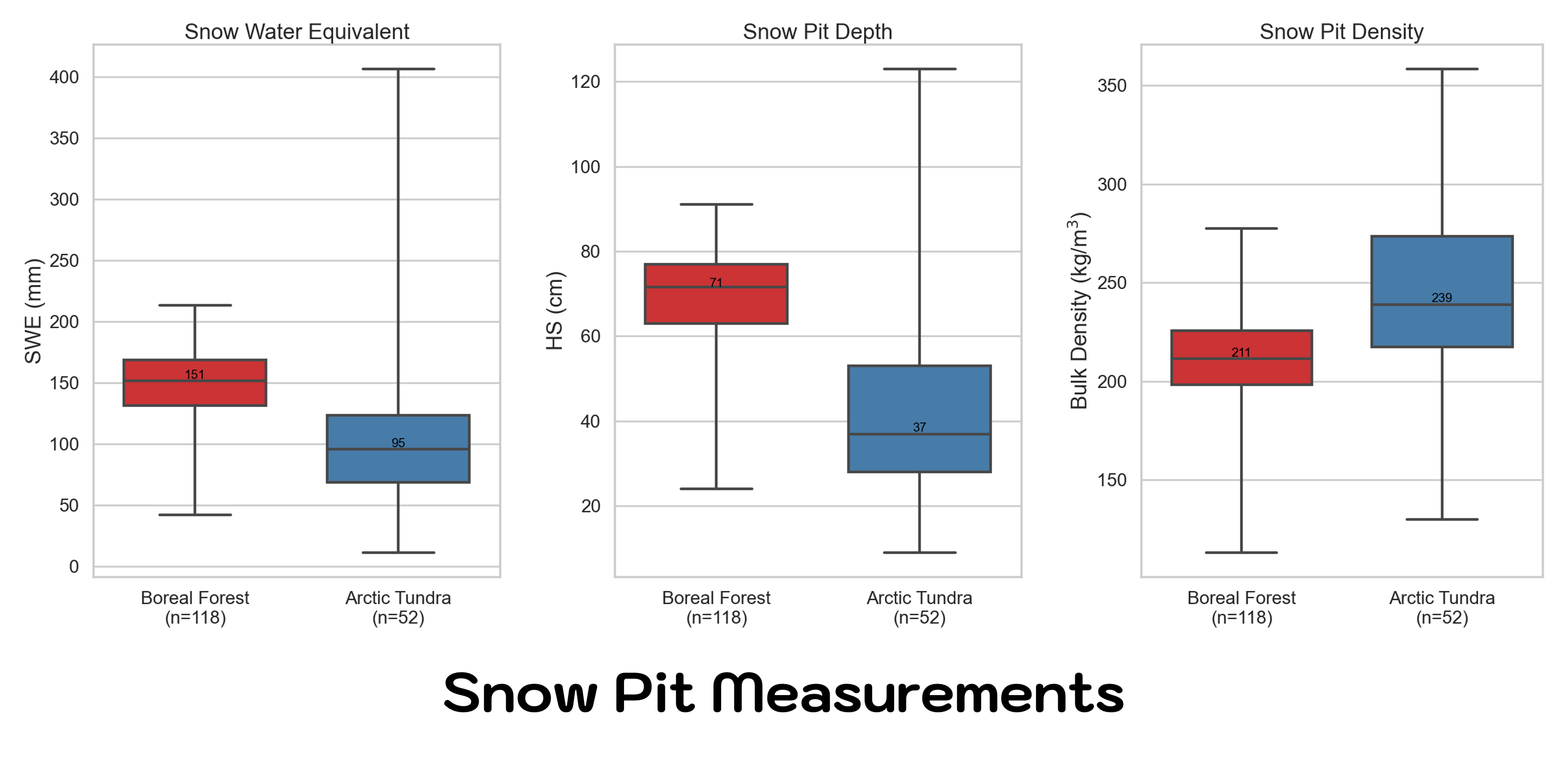
../../_images/967b2b7eb53056db560507981df7577b960307c2323c1b38891fc51876b90c69.png

We can compare our Adirondack snow sampler results to the snow pit measurement. The boxplots below were generated during the review and data submission preparation work for the March 2023 snow pits. Notice, the snow pit trends match those of the snow sampler tube. The median SWE is higher in the boreal forest as a result of the deeper snow. Overall, the tundra sites have greater density.

What are other ways to look at the data? Recall that the Boreal Forest has a land cover classification enbedded in the plot name. Why not look at SWE, depth, and density by land cover type? Recall, the Land Classification information is embedded in the pitID name (e.g. WB241 the ‘W’ stands for wetland, or EA221 the ‘E’ stands for Evergreen).

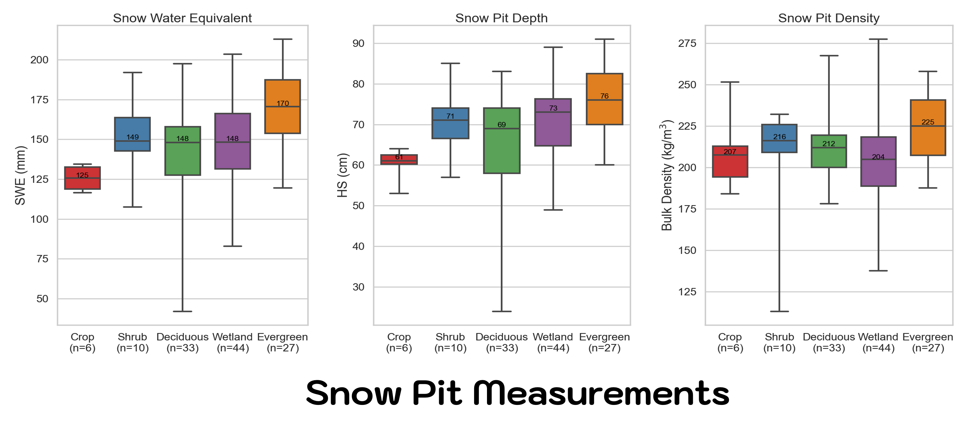
Does this mean that all Evergreen sites have more snow!?

Careful now, there is a lot to consider when interpreting results. This plot alone looks like we have deeper, denser snow in the Evergreen forests, but keep in mind you may not know the other environmental and terrain factors that might cause you to jump to this conclusion. Keep in mind relative location and elevation when looking at data. The Alaska study sites are all relativily flat compared to traditional complex terrain areas, but the majority of our Evergreen sites were sampled in the Caribou-Poker Creek Research Watershed, which is higher in elevation that the sites closer to Fairbanks.

Alaska was the last stop for SnowEx field campaigns, that means the data collection was easy-breezy.

WRONG.

Here are some challenges we encountered daily:

Ground vegetation - where is 0? Often, the bottom of the snowpack varied more than the snow surface!
Tussocks, what are they and why are there so many? (NOTE - tussocks were better quantified during the October sampling periods when snow was low.
Snow Voids - snowpack bottoms were not always flush to the ground surface and could be overestimated. Grassy vegetation mats, downed brush and shrubs, or other vegetation creates air pockets or vegetation gaps near the ground surface. Sometimes, the snow was suspended by 10-25 cm depending on the site.

These data are really exciting to look at because it’s the newest in the SnowEx collection following the Alaska campaign.

Let me introduce the snowexsql database by demonstrating how to run an example query. To work from the database, we are going to add some necessary imports.

Set Up Computing Environment#

#database imports
from snowexsql.db import get_db
from snowexsql.data import PointData, LayerData, ImageData, SiteData
from snowexsql.conversions import query_to_geopandas

The Basics#

How are the data contained?#

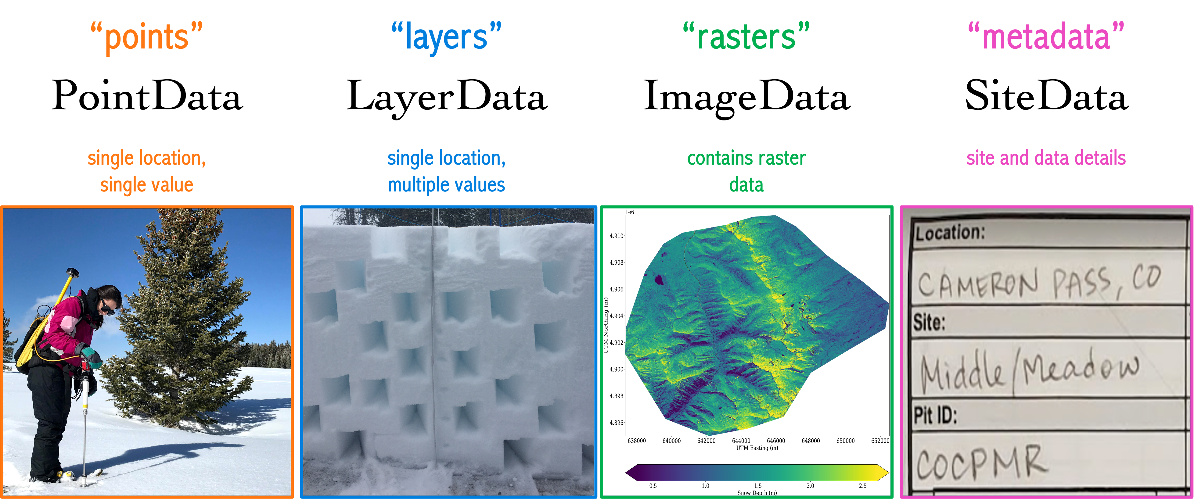
# load the database
db_name = 'snow:hackweek@db.snowexdata.org/snowex'
engine, session = get_db(db_name)

print('SnowEx Database successfully loaded!')

SnowEx Database successfully loaded!

What’s the first thing you might like to do using the database?#

Find overlapping data for data analysis comparison.

Example 1: Let’s find all the pits that overlap with an airborne sensor of interest.#

First, it would be helpful to know which of the airborne sensors are part of the database, right?

# Query the session using .observers() to generate a list
qry = session.query(ImageData.observers)

# Locate all that are distinct
airborne_sensors_list = session.query(ImageData.observers).distinct().all()

print('list of airborne sensors by "observer" name: \n', airborne_sensors_list)

list of airborne sensors by "observer" name: 
 [('USGS',), ('UAVSAR team, JPL',), ('ASO Inc.',), ('chris larsen',)]

Note: ‘chris larsen’ == airborne lidar data from Alaska

1a). Unsure of the flight date, but know which sensor you’d like to overlap with, here’s how:#

# Airborne sensor from list above
sensor = 'chris larsen' # Name given to Alaska Lidar data, observer Dr. Chris Larsen

# Form a query on the Images table that returns Raster collection dates
qry = session.query(ImageData.date)

# Filter for Alaska Lidar data
qry = qry.filter(ImageData.observers == sensor)

# Grab the unique dates
qry = qry.distinct()

# Execute the query 
dates = qry.all() 

# Clean up the dates 
dates = [d[0] for d in dates] 
dlist = [str(d) for d in dates]
dlist = ", ".join(dlist)
print('%s flight dates are: %s' %(sensor, dlist))

# Find all the snow pits done on these days
qry = session.query(SiteData.geom, SiteData.site_id, SiteData.date)
qry = qry.filter(SiteData.date.in_(dates))

# Return a geopandas df
df = query_to_geopandas(qry, engine)

# View the returned dataframe!
print(df.head())
print(f'{len(df.index)} records returned')

# Close your session to avoid hanging transactions
session.close()

chris larsen flight dates are: 2022-10-24, 2023-03-11

                             geom site_id        date
POINT (406069.144 7611197.807)     UKT  2023-03-11
POINT (438495.836 7775803.918)     ACP  2023-03-11
POINT (406060.880 7611607.651)     UKT  2023-03-11
POINT (438654.824 7776090.881)     ACP  2023-03-11
POINT (405487.123 7613118.982)     UKT  2023-03-11
records returned

1b).Want to select an exact flight date match? Here’s how:#

# Pick a day from the list of dates
dt = dates[1] # selecting the "2nd" date in the list, 203-03-11 during the March 2023 field campaign

# Find all the snow pits done on these days 
qry = session.query(SiteData.geom, SiteData.site_id, SiteData.date)
qry = qry.filter(SiteData.date == dt)

# Return a geopandas df
df_exact = query_to_geopandas(qry, engine)

print('%s pits overlap with %s on %s' %(len(df_exact), sensor, dt))

# View snows pits that align with first UAVSAR date
df_exact.head()

68 pits overlap with chris larsen on 2023-03-11

	geom	site_id	date
0	POINT (406069.144 7611197.807)	UKT	2023-03-11
1	POINT (438495.836 7775803.918)	ACP	2023-03-11
2	POINT (406060.880 7611607.651)	UKT	2023-03-11
3	POINT (438654.824 7776090.881)	ACP	2023-03-11
4	POINT (405487.123 7613118.982)	UKT	2023-03-11

1c). Want to further refine your search to select data from a specific Alaska study site? Here’s how:#

# Refine your search to Farmers Loop and Creamers Field
site = 'FLCF'
qry = qry.filter(SiteData.site_id == site)

# Return a geopandas df
df_exact = query_to_geopandas(qry, engine)

print('%s pits overlap with %s at %s' %(len(df_exact), sensor, site))

# View snows pits that align with first UAVSAR date
df_exact.head()

16 pits overlap with chris larsen at FLCF

	geom	site_id	date
0	POINT (467094.944 7194364.336)	FLCF	2023-03-11
1	POINT (467087.000 7194547.208)	FLCF	2023-03-11
2	POINT (467628.759 7194826.632)	FLCF	2023-03-11
3	POINT (467182.879 7194432.474)	FLCF	2023-03-11
4	POINT (467094.944 7194364.336)	FLCF	2023-03-11

1d). Have a known date that you wish to select data for, here’s how:#

# Find all the data that was collected on 3-11-2023 (i.e. the same day we selected airborne lidar data for)
dt = datetime.date(2023, 3, 11)

#--------------- Point Data -----------------------------------
# Grab all Point data instruments from our date
point_instruments = session.query(PointData.instrument).filter(PointData.date == dt).distinct().all()
point_type = session.query(PointData.type).filter(PointData.date == dt).distinct().all()

# Clean up point data (i.e. remove tuple)
point_instruments = [p[0] for p in point_instruments if p[0] is not None]
point_instruments = ", ".join(point_instruments)
point_type = [p[0] for p in point_type]
point_type = ", ".join(point_type)
print('Point data on %s are: %s, with the following list of parameters: %s' %(str(dt), point_instruments, point_type))

#--------------- Layer Data -----------------------------------
# Grab all Layer data instruments from our date
layer_instruments = session.query(LayerData.instrument).filter(LayerData.date == dt).distinct().all()
layer_type = session.query(LayerData.type).filter(LayerData.date == dt).distinct().all()

# Clean up layer data 
layer_instruments = [l[0] for l in layer_instruments if l[0] is not None]
layer_instruments = ", ".join(layer_instruments)
layer_type = [l[0] for l in layer_type]
layer_type = ", ".join(layer_type)
print('\nLayer Data on %s are: %s, with the following list of parameters: %s' %(str(dt), layer_instruments, layer_type))

#--------------- Image Data -----------------------------------
# Grab all Image data instruments from our date
image_instruments = session.query(ImageData.instrument).filter(ImageData.date == dt).distinct().all()
image_type = session.query(ImageData.type).filter(ImageData.date == dt).distinct().all()

# Clean up image data 
image_instruments = [i[0] for i in image_instruments]
image_instruments = ", ".join(image_instruments)
image_type = [i[0] for i in image_type if i[0] is not None]
image_type = ", ".join(image_type)
print('\nImage Data on %s are: %s, with the following list of parameters: %s' %(str(dt), image_instruments, image_type))

Point data on 2023-03-11 are: pulseEkko pro 1 GHz GPR, with the following list of parameters: density, depth, snow_void, swe, two_way_travel

Layer Data on 2023-03-11 are: , with the following list of parameters: density, grain_size, grain_type, hand_hardness, lwc_vol, manual_wetness, permittivity, temperature

Image Data on 2023-03-11 are: lidar, with the following list of parameters: depth

# fix this
qry = session.query(LayerData.value).filter(LayerData.type=='grain_type')
qry = qry.filter(LayerData.value=='MFcr')
count = qry.count()

print('The number of Layer Data containing melt-freeze crusts (MFcr) on %s are: %s' %(str(dt), count))

session.close()

The number of Layer Data containing melt-freeze crusts (MFcr) on 2023-03-11 are: 625

For more useful examples of querying and plotting please visit previous tutorial materials:#

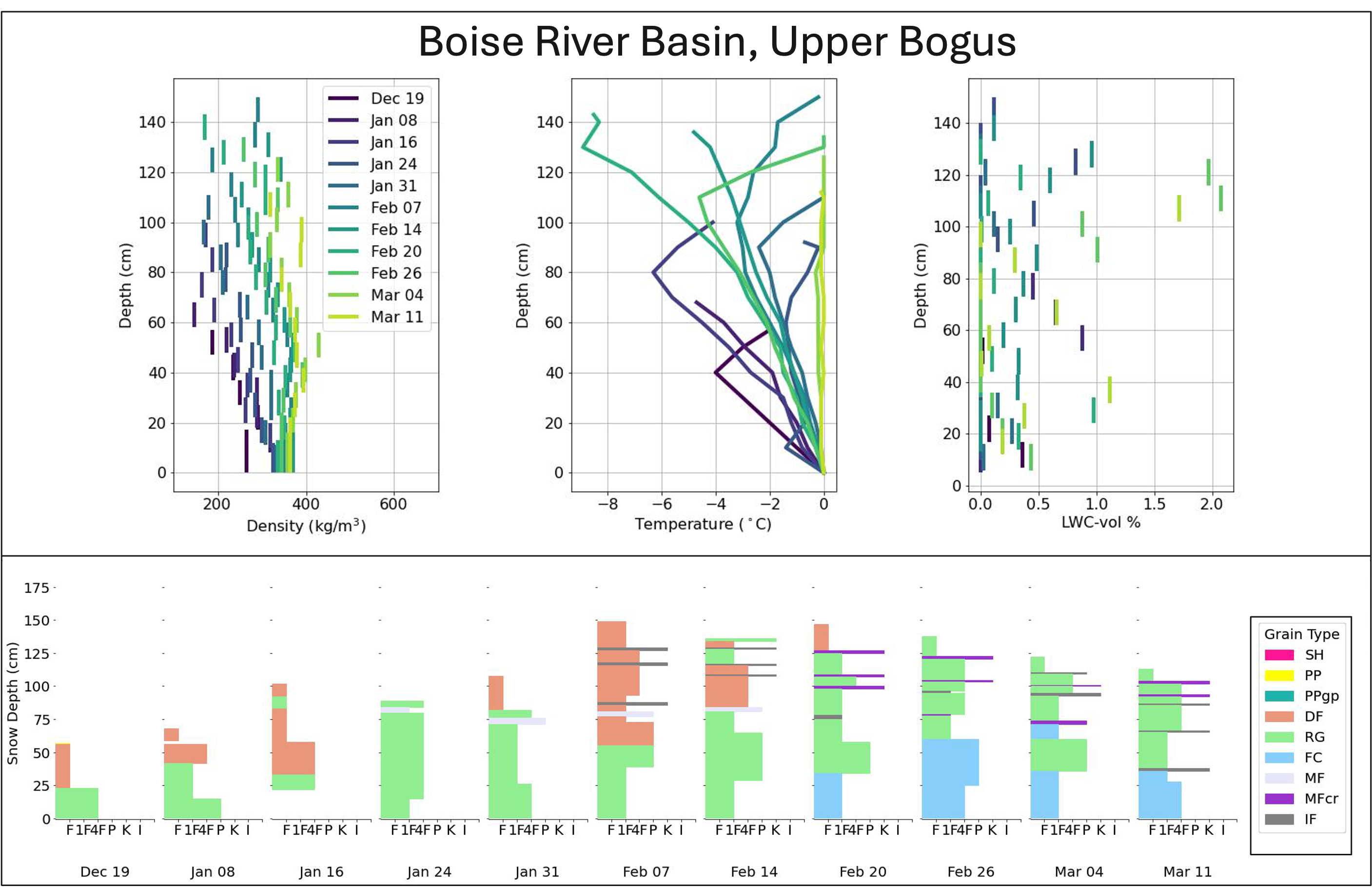
Hackweek 2022 - 03_snowex_database_preview (Examples #2 & #3)

Example #2 - plot snow depth profiles from open Time Series sites.
Example #3 - search for available liquid water content data through an interactive map.

PART II: Temporal Data (teaser)#

III: 2020/2021 Western U.S Time Series#

Objective - Explore data within the snowexsql database
Data description - weekly* snow pit data from multiple western U.S sites (*weekly does not apply perfectly to all sites).
Datasets -

Let’s conclude by studying this figure that captures weekly measurements from the Time Series (TS) campaigns. The Time Series field camapaign data products have matured since the last SnowEx Hackweek event.

Figure. Snowpack evolution at Bogus Basin (6,850 ft.) near Boise, Idaho. Top row: (left) - Density cutter measurements where the vertical bar shows 10 cm sample extent. (middle) - Snow temperature profile from digital thermometer. (right) - Liquid Water Content (LWC) measurements derived from A2 WISe sensor. Bottom row: Stratigraphy profile of snow according to grain type and layer hardness. Note the change in snow depth over time and the appearance of ice layers (IF) and melt-freeze crusts (MFcr) along with the transition from round grains (RG) to facets (FC).

Recap#

You know how to access NSIDC data and interact with 2017 & 2020 Grand Mesa and Senator Beck, Colorado SWE data.
You are aware of some general trends in tundra vs. boreal forest data and can form queries using the snowexsql database.
You have knowledge of what can be harnessed from the 2020 & 2021 Western U.S Time Series campaigns.

Data Exploration

Contents

Data Exploration#

PART I: Spatial Data#

I: 2017/2020 - Grand Mesa & Senator Beck, Colorado#

Download data from NASA’s NSIDC DAAC#

Let’s add some context to these data points#

Map + Imagery + Data#

What variability is there during the different sampling years?#

II: 2023 Arctic Tundra and Boreal Forest, Alaska#

Set Up Computing Environment#

The Basics#

How are the data contained?#

What’s the first thing you might like to do using the database?#

Example 1: Let’s find all the pits that overlap with an airborne sensor of interest.#

1a). Unsure of the flight date, but know which sensor you’d like to overlap with, here’s how:#

1b).Want to select an exact flight date match? Here’s how:#

1c). Want to further refine your search to select data from a specific Alaska study site? Here’s how:#

1d). Have a known date that you wish to select data for, here’s how:#

For more useful examples of querying and plotting please visit previous tutorial materials:#

PART II: Temporal Data (teaser)#

III: 2020/2021 Western U.S Time Series#

Recap#